Exporting results
In this section, we’ll learn how to export the generated results from the GLOSSA analysis, understand the structure of the downloaded files, and show tips for working with these files.
The export form
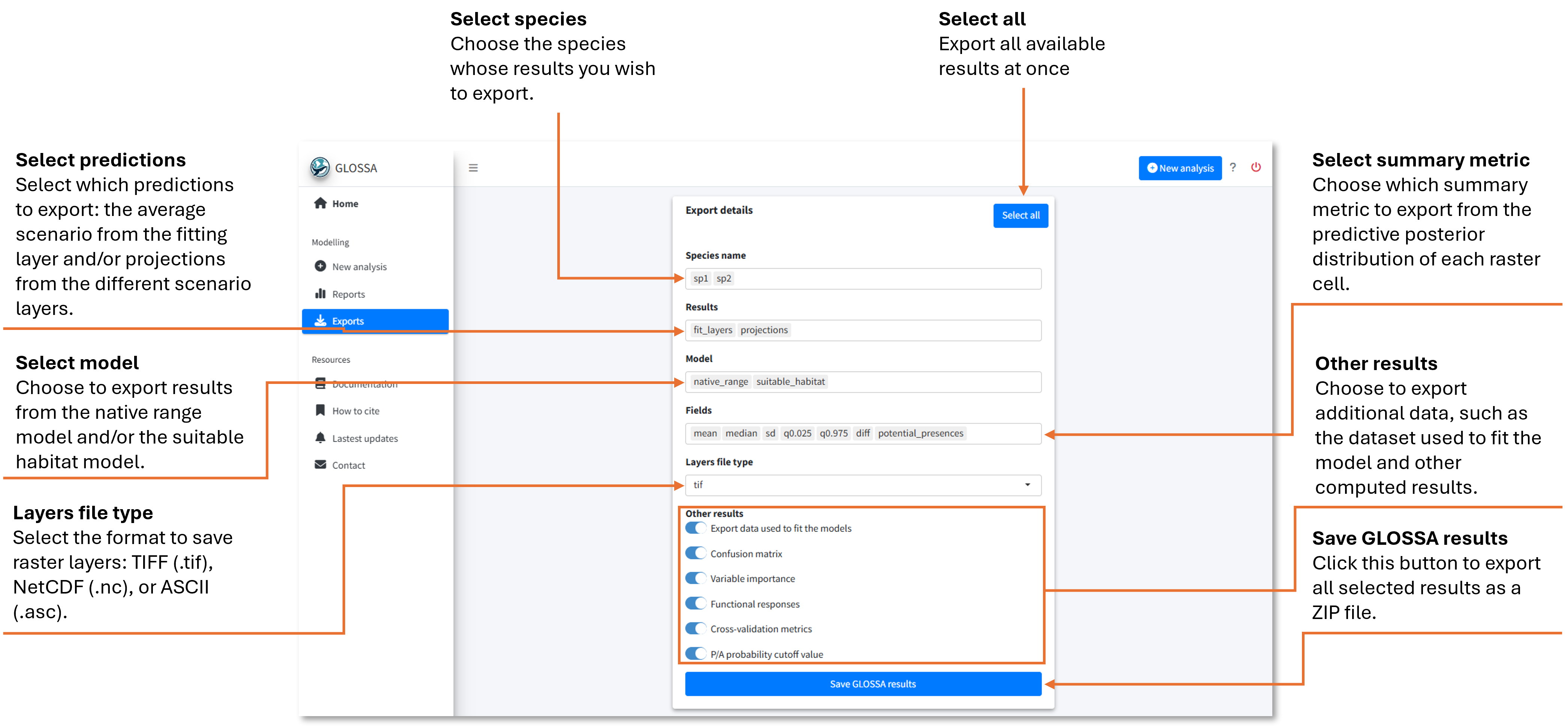
When opening the Exports tab, you’ll find a form to select which results to export. This form provides access to all results displayed in the Reports tab, as well as the data used to fit the models.

In the first field, select the species or occurrence files you want to export—multiple species can be chosen. In the second field, choose which prediction results to export: either the predictions based on the average environmental scenario used to fit the model or predictions from the different projection layers. Next, decide whether to export the results for the native range (NR) model, the suitable habitat (SH) model, or both.
Since GLOSSA operates within a Bayesian framework, each grid cell has an associated predictive posterior distribution. In the Fields field, you can choose which summary statistics to save:
- mean: mean value
- median: quantile 0.5
- sd: standard deviation
- q0.025: quantile 0.025
- q0.975: quantile 0.975
- diff: difference between quantile 0.975 and 0.025
- potential_presences: predicted presences (
1) and absences (0) using the estimated optimal cutoff.
For these raster files, you can select the file type in the next field (TIFF, NetCDF, or ASCII).
Additionally, you can export other data, such as:
- The processed data used to fit the model
- The confusion matrix of predicted vs. observed occurrences
- Variable importance scores
- Functional response plots
- Cross-validation metrics
- The value of the estimated probability cutoff for presence/absence.
If you want to export everything, use the Select All button.
Once you have selected what you want to export, click on the Save GLOSSA Results button. A ZIP file containing all selected results will be downloaded to your local machine.
Exported ZIP file
When you export results from GLOSSA, a ZIP file is created that organizes the outputs in a structured way, making it easier to explore specific files and load them into R for further analysis.
ZIP file overview
The ZIP file is organized by species, with a folder for each species or occurrence file you analyzed (e.g., sp1, sp2). Within each species folder, there are several subfolders and files containing specific results:
- sp_model_data.csv: A tab-separated file with the dataset used to fit the model after processing the data (
decimalLongitudeanddecimalLatitude: longitude and latitude from the occurrence file.,timestamp: timestamp values,pa: response variable indicating presence or absence,Xs: one column per uploaded predictor variable,grid_longandgrid_lat: longitude and latitude from the raster created for the native range model). - sp_presence_probability_cutoff.csv: Estimated optimal probability cutoff for presence/absence prediction for both the native range and suitable habitat models.
- confusion_matrix: Contains tab-separated files (NR and SH) with confusion matrices for each model, comparing observed occurrences with predicted values and probabilities.
- cross_validation: Includes tab-separated files (NR and SH) with cross-validation results for \(k = 10\) folds, one row per fold.
- functional_responses: Contains one tab-separated file per predictor variable in the suitable habitat model, with partial dependence plot values. Each file includes a column with talues of the predictor variable used to construct the plot and the probability values (mean and quantiles 0.025 and 0.975 columns) that represent how predictor variables influence the model, that is, the changes relative to the overall central tendency.
- native_range and suitable_habitat: These folders contain raster files with predictions for each model type (native range and suitable habitat), organized as follows:
- fit_layers: Results from the fitting dataset, organized by summary statistics:
- diff: Difference between the 97.5th and 2.5th quantiles.
- mean: Mean prediction value.
- median: Median prediction (quantile 0.5).
- potential_presences: Binary presence-absence predictions based on the optimal cutoff.
- q0.025 and q0.975: Lower and upper quantiles of the posterior distribution.
- sd: Standard deviation.
- projections: Contains projections for each environmental scenario (e.g.,
project_layers_1,project_layers_2), with the same summary statistics as above.
- fit_layers: Results from the fitting dataset, organized by summary statistics:
- variable_importance: Contains a tab-separated file for each model (NR and SH) listing the variable importance score for each predictor variable. Each row represents one of the 10 permutations performed.
Working with the exported Files in R
All the exported files are in tab-separated format except for raster files, which are saved in the format you selected. You can load the CSV files into R with the read.csv() and read.table() functions, and raster files with the rast() function from the terra package. For example:
# Load functional responses
functional_responses <- read.table("path/to/sp1/functional_responses/sp1_functional_response_x1.csv", header = TRUE, sep = "\t", dec = ".")
plot(functional_responses$value, functional_responses$mean)

# Load projection file
library(terra)
projection <- rast("path/to/sp1/suitable_habitat/projections/project_layers_1/mean/sp1_suitable_habitat_projections_1_mean.tif")
plot(projection)If you’re exporting data for multiple species or comparing models, automating workflows in R can streamline your analysis.
Conclusion
Congratulations! You’ve now learned how to run a complete analysis with GLOSSA, from data preparation to output export. Now it’s time for you to try it with your own data! To explore more tutorials or real case examples, visit Tutorials and Examples.